Models are useful. They help us understand the world around us and aid us in predicting what will happen next. But it’s important to remember that models don’t necessarily reflect the underlying reality of the thing we’re modeling. The Ptolemaic model of the solar system assumed the Earth was the center of everything but in spite of that spectacular error, it did a good job of predicting the motions of the stars, planets, moon, and sun. It was the best model available for over a thousand years. But new data (e.g., phases of Venus as revealed by Galileo’s telescope) and errors in predicting the motions of the planets demonstrated that the sun-centric Copernican/Kepler models were superior.
There are a lot of models for the Cboe’s VIX. None of them are particularly good at predicting what the VIX will do tomorrow but they can be useful in predicting general behaviors of the VIX. The most popular model for the VIX (although people might not recognize it as a model) is simple mean reversion.
Simple Mean Reversion
Car gas mileage is a good example of a simple mean reverting process.
Over time your car’s gas mileage will exhibit an average value, e.g., 28 miles per gallon. You don’t expect to get the same mileage with every tank because you know that there are factors that make a difference with your mileage (e.g., city vs highway driving, tire air pressure, and wind direction) but over time you expect your mileage to cluster around that average value. If you get 32 miles per gallon on one tank of gas you reasonably expect that next time you check it will likely be closer to 28. If the values start varying significantly from the average you start wondering if something has changed with the car itself (e.g., needs a tune-up)
A mean-reverting random walk is a relatively simple model and fits some of the basic behaviors of the VIX. Specifically, over time the mean value of the VIX has stayed stable at around 20 and the VIX exhibits range bound behavior—with all-time lows around 9 and all-time highs around 80.
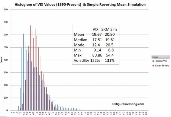
However, there are many aspects of the VIX that aren’t well explained by a simple mean-reverting model. For example, a simple mean reverting process will have its mode value (the most frequently occurring values) close to its mean. This is not the case of the VIX; its mode is around 12.4—a long way away from its mean. The histograms below show that difference visually.
Another VIX behavior that departs from a simple mean-reverting process is the abrupt cessation of values below 9—almost a wall. For a normal mean reverting process you would not expect such a sharp cut off at the low end.
The Acid Test: How good is the model for predicting the future?
Having a good model for a process is useful because it can help us predict at least some aspects of the future. For example, we can use our average gas mileage to decide whether we need to gas up before entering a long stretch of highway without gas stations.
A simple mean-reverting model is not particularly good at predicting the future moves of the VIX. If the VIX is low (e.g., 12 or below) a simple mean-reverting model predicts that since the VIX is far from its mean that will likely increase soon. But history shows this is usually not the case. Often the VIX can be quite content to hang around 12. This leads to news stories quoting various pundits stating “The VIX is broken” –when in reality they are just using an inferior model.
As I said earlier there are VIX models out there that address some of these deficiencies. Unfortunately, the ones I know of are complex and not very intuitive. I believe the model that I describe below can improve our intuition considerably without adding too much complexity.
A Better VIX Model
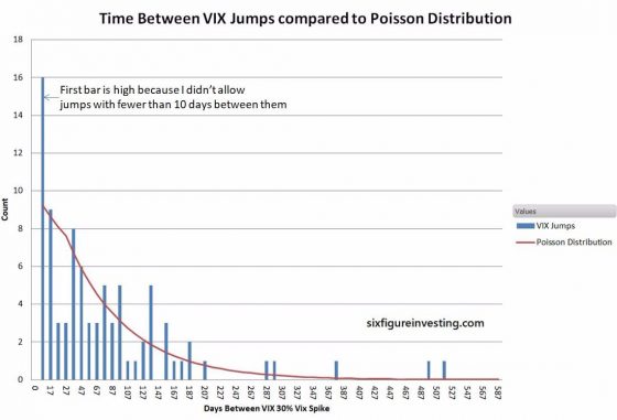
A better way to view the VIX is that it behaves like the combination of two interacting processes: a specialized mean reverting process and a “jump” process. The jump process captures the behavior that all VIX watchers know—its propensity to occasionally have large percentage moves up and down. Since 1990 there’ve been over 86 times where the VIX has increased 30% or more in a 10 day period. The occurrence of these spikes is effectively random with a probability of happening on any given day of around 1.28%. It’s like a roulette table with 78 slots, 77 of them black and one red. If the ball lands on a black the normal reigns—if red then things get crazy. The graph below shows a histogram of the number of days between these 30% spikes in the VIX since 1990.
There’s nothing that prevents reds on consecutive spins nor is there some rule that reds become really likely if you haven’t had a red in a while. The roulette ball has no memory of where it landed on previous spins.
VIX jumps are generally not just one-day events; subjectively it looks like it takes around two weeks before the market reverts to more typical behavior. The model assumes that when a jump occurs it essentially drives the behavior of the VIX for 10 trading days.
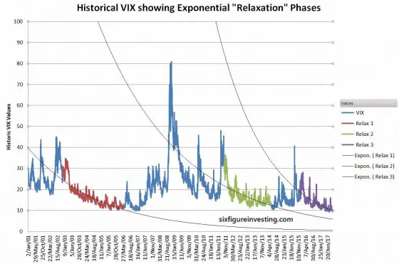
The other process, the specialized mean reverting process, addresses the non-jump mode of the VIX—which is historically around 85% of the time. One of the key behaviors it needs to address is the slow relaxation in the mean value of the VIX after a big volatility spike rekindles a generally fearful attitude in the market. This decay process continues (unless interrupted by another VIX jump) until the average monthly VIX values drop into the 11-12 range.
The chart below illustrates this relaxation process.
This characteristic can be modeled by expecting the short term mean of the VIX (when it’s not jumping) to decay exponentially until it reaches its “quiet” mean of around 11.75. It works well to quantify this decay as having a time constant of 150 days.
With this approach, sans jumps, the difference between the current VIX value and its long-term quiet value will decay by 50% in 104 days. So if the VIX is at 30 the model predicts the mean will decline to 20.75 in 104 days [30- (30-11.5)*0.5=20.75]. If there are no jumps for the next 104 days the VIX’s mean would decline to 16.13. If a jump occurs in the interim the short term mean is reset to the VIX’s value at the end of the jump.
The other part of the specialized mean reverting process mimics the day-to-day volatility of the VIX. I used a formal mean reverting diffusion process (Ornstein-Uhlenbeck) to accomplish this. Despite its scary name, you can think of it as a random walk with the thing “walking” being attached to the mean with a spring—similar to walking a dog with a springy leash. The further the dog gets from you the larger the force pulling the dog back to you.
Unlike the simple mean-reverting model often used for the VIX, this process has a much tighter distribution, with the extreme values effectively limited to around +-20% from the mean. When the VIX is quiet this process replicates the firm lower limit on the VIX, a VIX of 9 is -21.74% lower than a quiet mean of 11.75.
Simulating the Model
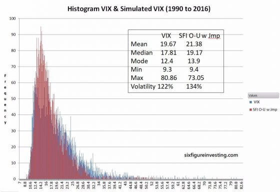
To implement/validate this model I estimated the key input variables and then used Excel to simulate 20-year volatility sequences. I then compared these time series to the actual VIX history and tuned the model’s parameters such that the key characteristics (e.g., volatility, mean, mode, decay rates) were similar to the VIX’s historic values.
Resulting histogram of historic VIX values vs the simulated combined process
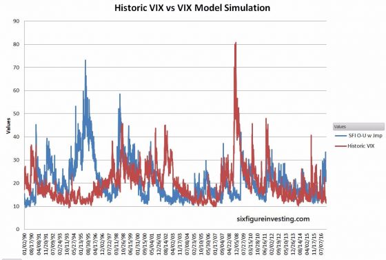
The next chart shows an example 20 year time series of the simulated VIX combined process compared to the historic VIX. The two series aren’t time synchronized; my intent is to show how the simulated VIX time series has the same visual feel as the real VIX.
Conclusion
This improved model is not a path to riches. It isn’t any better than other models at predicting when VIX jumps will occur. However, this model does help us understand how the VIX behaves over longer time spans. In particular, during times of sustained low volatility, it predicts that the VIX will tend to stay low until the next significant VIX spike and not trend up like the simple mean-reverting model demands.
Quant Corner
- The mean-reverting diffusion process used is an Ornstein-Uhlenbeck mean reverting diffusion process using a log-normal distribution. The volatility was set at an annualized 112% and the return to mean strength parameter ETA set to 0.3. The mean of the process is determined by the previous day’s VIX value minus the exponential decay factor that will decay the mean down to 11.75 over time if there are no additional jumps (Tau of 150 days). If the mean has decayed down to 11.75 the process acts very similarly to the VIX’s low volatility regimes (e.g., 2004-2006, 2016-2017) with the “return to mean” factor effectively acting to keep the VIX higher than 9.0
- The Jump process used (with a few small tweaks) is a compound Poisson process where the probability of a jump sequence is random with a probability of a jump being 1.28% per day. The jump sequence and its daily amplitudes are determined using a technique borrowed from rappers called sampling. Instead of trying to recreate the decidedly non-Gaussian distribution of VIX jumps I reused historic VIX jumps by randomly selecting, and replaying one of the more than 85 jump sequences since 1990 where the VIX jumped more than 30% in 10 days. Each jump sequence is 10 days long, with the first 2 days being the behavior before the jump.

Very interesting findings!
I am curious the relaxation model: if the relaxation is exponential decaying (at time_constant=150), what is the process that ramping up to the next “jump”? I understand there is almost a sharp cutoff to the left of the mode in Figure 1. But it seems there is another process kicking in before the next jump (I was looking at the curve between the red segment and the next peak).
Not sure which chart you’ll referring to — “Historical VIX showing Exponential ‘relaxation” phases”? I don’t think there is a consistent run-up mechanism except for “known unknown” sorts of run-ups for things like Brexit, elections. I’d love it if there was one because it would make holding short volatility positions a lot less scary.
The model treats jumps as random events with unpredictable timing (other than Poisson distribution) and no warming.
right, I referred to “Historical VIX showing Exponential ‘relaxation” phases”. Ok, that’s fine if you don’t see any trace there. I was thinking may be able to use some learning algorithms to trace the jumps.
By the way, have you thought about why the time constant is 150-day? Is this number related to seasonality events like “Sell in May” and “January Effect” (they are about 30-week)? I assume your chart was based on some indeces, right? So if plotting individual stocks, I would expect the time constant to be about 70-day due to earnings. Is this reasonable?
Hi Hans, I came up with the 150 day number emperically. Using my model I I forced it to use the actual VIX spikes in the order that they arrived historically, then I adjusted the time constant until the decay shown in my model closely matched the historical decay rates of the VIX.
Ok, thanks Vance. Now I see how you got the 150 number. Great work!
Vance – is there a way you might be able to show the poisson histogram chart for the number of days between vix spikes of 1) at least 10% and 2) at least 20%? the 30% chart is awesome btw.
Hi EC, I think 10% would be way too noisy but I’ll try to do the 20% point threshold. Probably will be a while.
Hi Vance, great research, good collection of resources. I am trying to diversify my portfolio away from being mostly in short volatility products like SVXY and XIV into other asset classes. Towards that end, I am trying to find other futures markets whose term structures resemble the term structure of VIX – mostly in contango except for occasional spikes in the spot price. Do you know of any other products/assets with a futures term structure that fits the criterion and which has exchange traded products that take advantage of this term structure?
Of course, the term structure does not have to be mainly in contango either. If it is always (or most of the time) in backwardation that will work too. But mostly, what I see is futures term structures with no distinct structure, or which change too frequently from contango to backwardation and back again based on unpredictable extraneous factors (crude oil futures being a prime example of this type of behavior).
Thank you very much, and please keep up the good work!
Vance, another great article. Keep up the good work!
very interesting. i am still a bit fuzzy on the modelling when vix is below 11.75 (mean). can you give a simple numerical example of when vix is say 9.5?
Hi EC, If the VIX has decayed to its quiet mean of around 11.75 then there are mean reverting random moves around that mean. If VIX is at 11.75 then the next day’s percentage moves can be modeled with a normal distribution with a mean of zero and a daily volatility of around 6%. 68% of the time the move away from 11.75 will be +-6% or less. The mean version factor ETA sets the magnitude of the mean reversion force that tends to drive the process back to its mean. By the time VIX is near 9.5 it would take a high sigma event in the right direction to drive the VIX lower still–otherwise, the next day’s random move + the mean reversion ETA factor times the difference between the “quiet” mean and the current value will generally drive the VIX value up.
Vance
thanks. very helpful. appreciate all the great insights on your site!
This is a great article Vance. Thanks for sharing your research! It’s intuitive and makes great sense in terms of how humans react to fear and greed. Now…. if you will just come up with a model on when those jumps will happen, we’ll be all set! 🙂
I do have one other question for you – especially if you’re curious to tackle a new angle regarding volatility prediction… Have you ever tried to determine if the diffusion across sectors in a given index has any predictive effect on the overall index volatility? (so for example: let’s say the returns between the energy sector and the technology sector have been significantly different over the last 3 months. Does that diffusion level play into overall market volatility for the next month? ) I’d love to hear your thoughts…
Hi Lee, Could you say more about diffusion between sectors? I suspect sector rotation is normally modeled as more of a mean reversion process but “diffusion” sounds more like a random process.
Apologies for taking so long to reply – I built a new PC, and didn’t get any type of email notification…. Diffusion may have been a poor choice of words on my part – lack of correlation (or even negative correlation) between sectors may have been a better choice…. The real question going through my mind is whether or not the sectors that make up the S&P 500 are a bit less correlated at present – if that’s the case, then you could have a relatively high level of volatility in a given sector (or at the individual stock level), and still have low volatility for the S&P 500 at the index level. The rational would be that one sector could go up, another one could go down, and the index would stay (relatively) flat. I’m not sure that this would necessarily provide any type of edge, but…. I think I’d feel more confident that the index may not move as much if things underneath the surface are still at more normal levels of volatility. Why? Well…. if every stock has just lost volatility (as measured by IV), then it feels like anything that scares investors in general could really prompt a VIX spike. Just musing…
Nice work, thank you.
Hi Vance. I am new to your site and trading as well. A few days ago I read from another blogger that the direction of the vix could be predicted by just applying a 10 day simple moving average to its slope. In other words when vix is below its 10 sma, go long svxy or xiv or spy; and when vix is above its 10 sma the author advises to buy uvxy or vxx. Do you have any idea about that?
Also I appreciate your article and would like to know if it’s possible to transform it into a trading system?
Thanks
Hi Plok, In general I’m not a fan of moving average type approaches. They will work some of the time but usually not over the long term. If you methodically look at how they perform over a couple of years they are usually disappointing.
My model describes general trends in the VIX but it can’t predict when volatility will spike–which is the most important problem with volatility trading.