It was not obvious (at least to me) that volatility theoretically scales with the square root of time (sqrt[t]). For example, if the market’s daily volatility is 0.5%, then theoretically the correct value of volatility for two days is the square root of 2 times the daily volatility (0.5% * 1.414 = 0.707%), or for a 5 day stretch 0.5% * sqrt(5) = 1.118%.
This relationship holds for ATM option prices too. With the Black and Scholes model if an option due to expire in 30 days has a price of $1, then the 60 day option with the same strike price and implied volatility should be priced at sqrt (60/30) = $1 * 1.4142 = $1.4142 (assuming zero interest rates and no dividends).
Underlying the sqrt[t] relationship of time and volatility is the assumption that stock market returns follow a Gaussian distribution (lognormal to be precise). This assumption is flawed (Taleb, Derman, and Mandelbrot lecture us on this), but general practice is to assume that the sqrt[t] relationship is close enough.
I decided to test this relationship using actual S&P 500 data. Using an Excel-based Monte-Carlo simulation1 I modeled 700 independent stock markets, each starting with their index at 100 and trading continuously for 252 days (the typical number of USA trading days in a year). For each day and for each market I randomly picked an S&P 500 return for a day somewhere between Jan 2, 1950 and May 30, 2014 and multiplied that return plus one times the previous day’s market result. I then made a small correction by subtracting the average daily return for the entire 1950 to 2014 period (0.0286%) to compensate for the upward climb of the market over that time span. Plotting 100 of those markets on a chart looks like this:
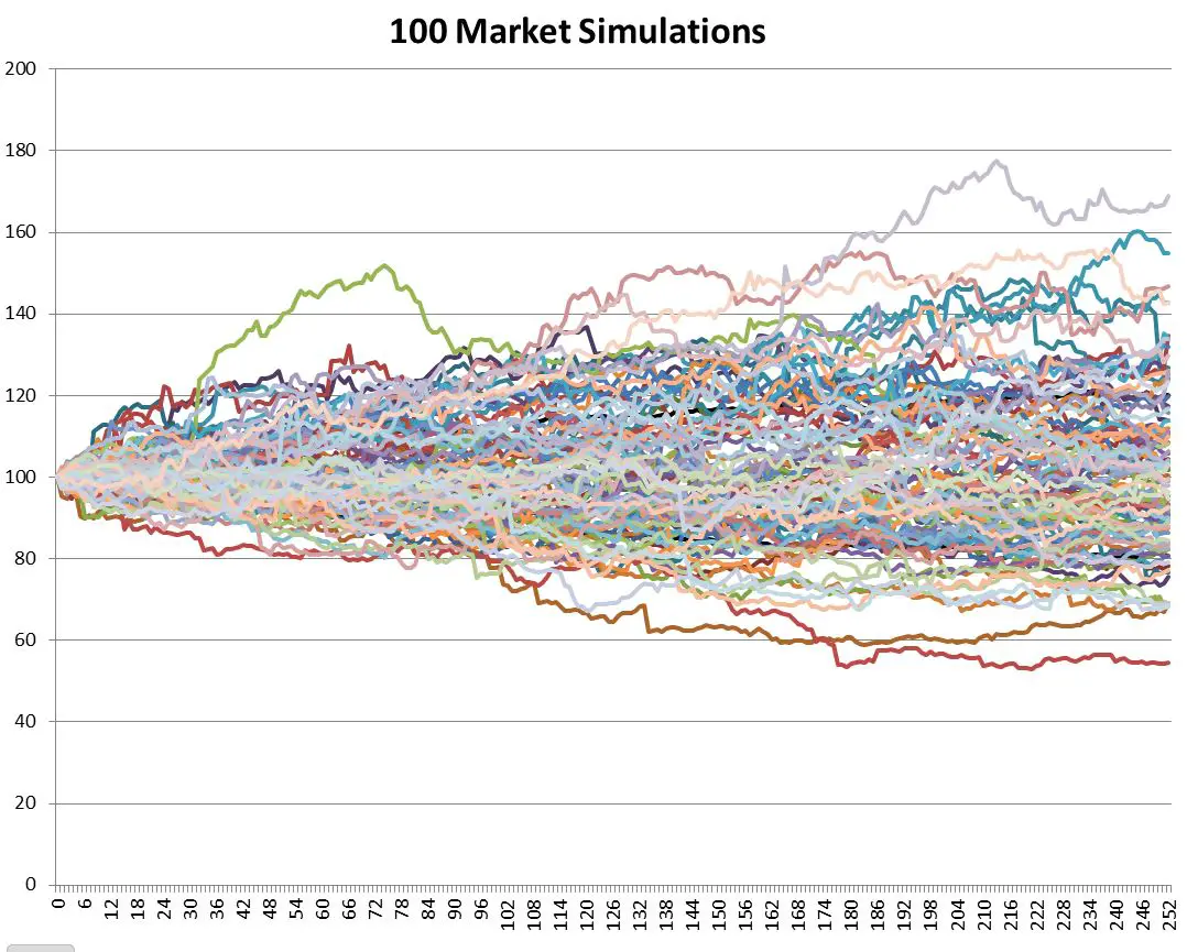
Notice the outliers above 160 and below 60.
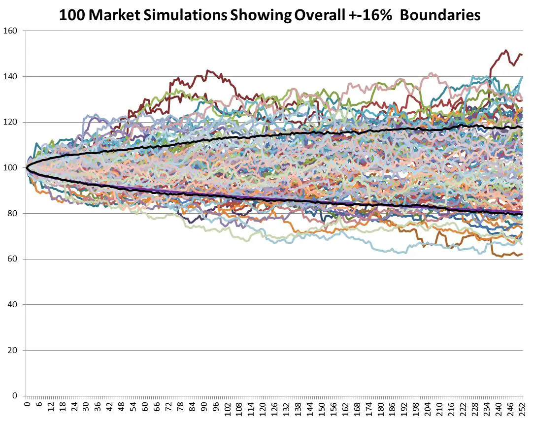
Volatility is usually defined as being one standard deviation of the data set, which translates into a plus/minus percentage range that includes 68% of the cases. I used two handy Excel functions: large(array,count) and small(array,count) to return the boundary result between the upper 16% and the rest of the results and the lowest 16% for the full 700 markets being simulated. The 16% comes from splitting the remaining 32% outside the boundaries into a symmetrical upper and lower half. Those results are plotted as the black lines below.
The next chart compares those two lines to the theoretical result which takes the annualized standard deviation of the S&P 500 daily returns from 1950 to 2014 and divides it by the square root of time.
Standard Deviation (N) = Annualized Standard Deviation/ sqrt (252/N)
Where N is the Nth day of the simulation.
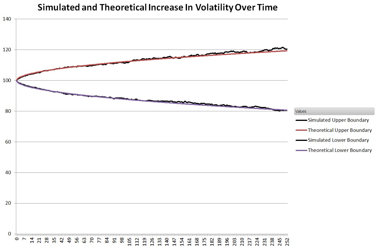
Impressively close.
Since the simulated boundaries vary some from run to run I collected 32 runs and determined the mean
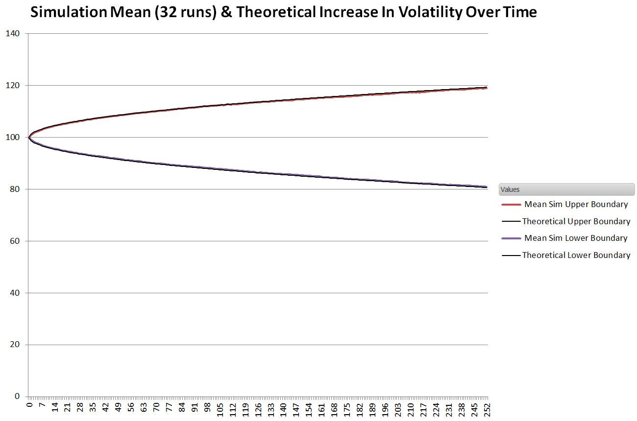
Very, very close.
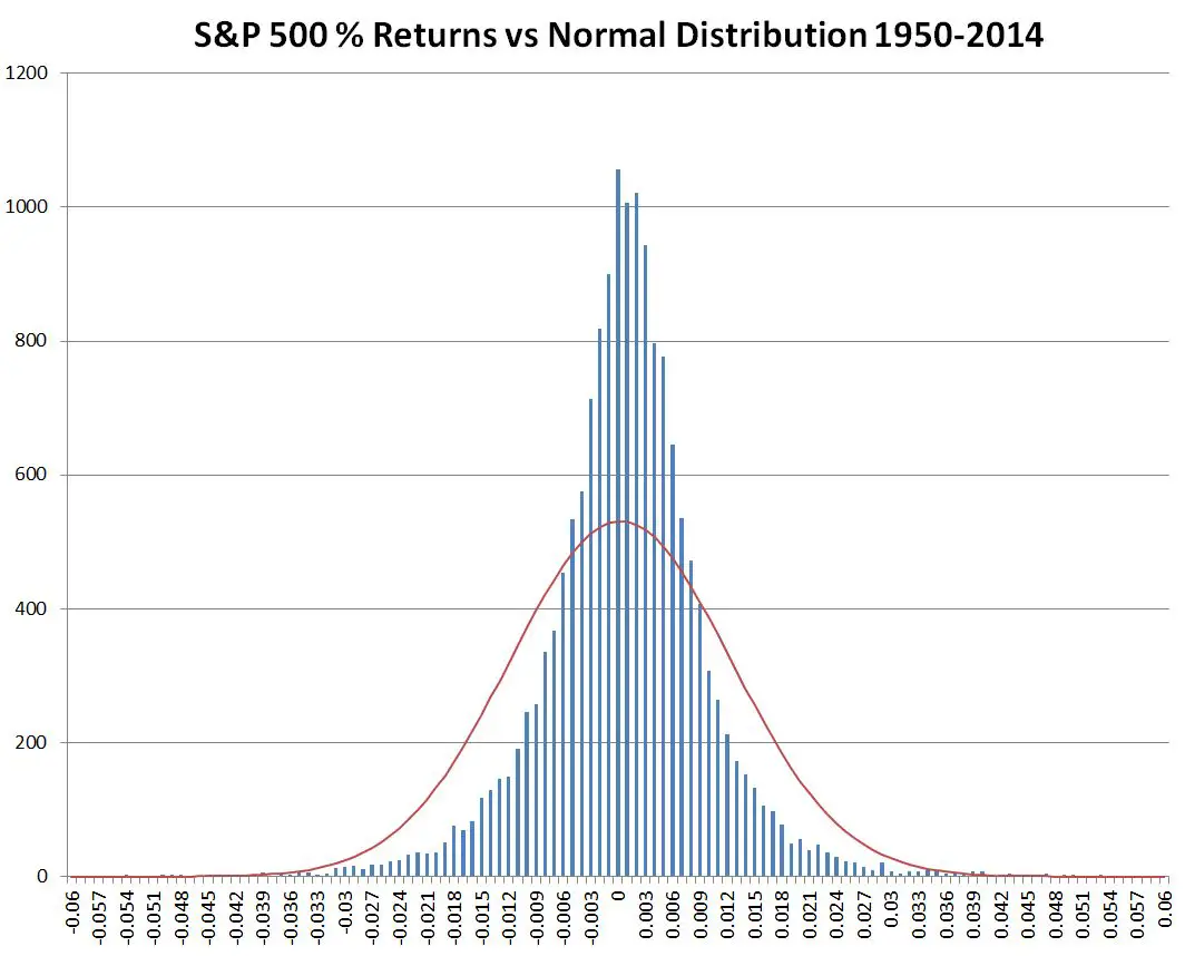
So, in spite of the S&P 500’s distribution of results not being particularly normally distributed (see chart below), the general assumption that volatility scales with the square root of time is very appropriate.
Notes:
- Returns are expressed as the natural log of the current day’s close divided by the previous day’s close. The specific daily return used is selected by randomly choosing a number between 0 and 16204 (Trunc(Rand()*16205)) and then using that number to index into the table of SPX returns. The 16205 constant is the number of trading days from 3-Jan-1950 to 30-May-2014. As mentioned in the post, the overall daily mean for that period (0.0286%) is subtracted from the result to compensate for the general upward bias of the market over that period.
I read that Albert Einstein originally discovered the sq rt law of distance linear relationship to sqrt of time. It was related to a study of thermodynamics, in which Delta T across a material subjected to a heat source was determined to be proportional to distance from heat source, and that was being studied to prove that materials are made of molecules circa 1930. Einstein discovered the proportionality to sq rt time by studying displacement of cells in Brownian movement. … In determining projected profit from Selling naked calls , I was dividing premium by time to eXP for profit per day, but I am considering switching to premium/ sq rt days to exp. Your thoughts? REF: Drunken Sailor model: A drunken sailor stumbles out of a bar, and wanders aimlessly trying to go home. Distance from bar is observed to be proportional to sq rt of Time, same as Brownian motion. This ends up as a component of BS option pricing formula
Hi Phil, As you say, the 1/sqrt(time) behavior of time decay is baked into the B&S model. I’ve never gone into analytical mode on it, but my sense is that the standard equations overestimate theta decay during the last few days before expiration. Options can have significant amount of premium left on them the day of expiration which can be pretty frustrating if you’re short. My guess would be sqrt(t) would be better than a linear model. I know with VIX options they have a somewhat different theta profile, where decay is more logarithmic as opposed to sqrt(t). This gives a characteristic where the theta drop is quite low until you get quite close to expiration, and then it exponentially down to zero at the end.
Best Regard, Vance
volatility scaling by sqrt(T) is mathematical identity for independant samples. var(a+b) = var(a) + var(b)
so not sure what this analysis really proves. since you made the each sample independant (by choosing it randomly from large sample), you are supposed to get this result just by design.
Looks to me this is more of a illustration of central limit theorem as you used the properties of normal distribution in calculating your sigma (if the 1yr return distribution was not normal, 68% of the sample would not define sigma).
The distribution of the S&P 500 returns are not normally distributed. I can imagine non-normal distributions (e.g. those with power law tail distributions) where randomly selecting samples would not lead to a square root of time change in volatility, but in the case of the S&P it does closely follow that behavior. I computed the sigma as if the distribution was normal, and compared it to a model free distribution of paths from the simulation.
— Vance
From Morningstar, on this subject:
http://corporate.morningstar.com/US/documents/MethodologyDocuments/MethodologyPapers/SquareRootofTwelve.pdf
Exactly. So if the returns are logarithmic, they are additive and the sqrt of 12 works fine. And it required only i.i.d, with distribution not necessary normal.
>the general assumption that volatility scales with the square root of time is very appropriate.
Nope. The assumption that volatility scales with the square root of time for series of randomly sampled returns is appropriate. But returns in the real world are not randomly sampled from some distribution, they are path-dependent.
James Mai talks a bit about this in Hedge Fund Market Wizards, specifically regarding trends (long-term they cause the square root estimate to be too low), but there are other effects at play, as well.
Could you point me to anything supporting path dependency, say, for stocks data? As far as I know, GARCH doesn’t show any.